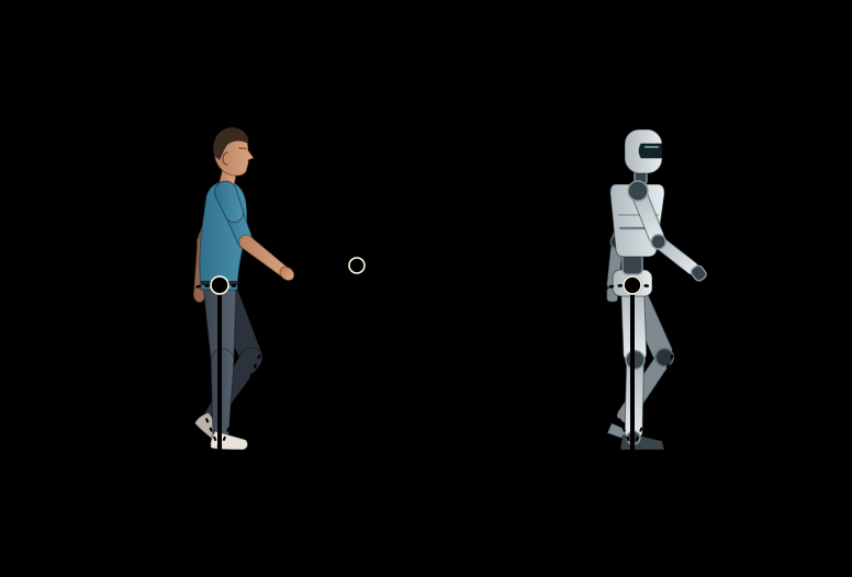
Two ways to move on two legs
You walk without thinking about it, yet every step is a small piece of applied physics. When you walk, your body vaults over a stiff leg; when you run, it bounces on a leg that works like a spring. These two tricks save energy in different ways, and the same two are used by animals as different as turkeys, dogs and kangaroos 1. Walking and running, the two basic gaits of humans, are very complex movements – but they can be described with two simple models: an inverted pendulum and a spring 2.
Walking upright on two legs is old: striding bipedalism may have originated soon after the lineages of humans and chimpanzees split. Running long distances came later; according to Dennis Bramble and Daniel Lieberman, endurance running is a capability of the genus Homo that originated about 2 million years ago and may have shaped the human body 3.
This article explains how the pendulum and the spring work, why you switch from walking to running at about the same “speed number” as a child, an adult or a person in simulated low gravity – and how engineers build and train robots that walk on two legs. The same kind of number – a Froude number – also sets the rhythm of a cat’s tongue in How cats drink.
One step in four phases
- Heel strike. The front foot lands while the back foot is still on the ground. For a moment both legs carry the body, and its path must be redirected from going down to going up 4.
- Vaulting. The back foot leaves the ground and swings forward. The body vaults over the almost straight stance leg; it slows down as it rises and is highest in the middle of the step 5.
- Falling forward. Past the top, the body falls forward and down on its arc and speeds up again. Potential energy turns back into kinetic energy 1.
- Push-off. The calf muscles and the Achilles tendon push the foot off the ground, while the other foot lands – and the next pendulum swing begins 6.
Biology lens: springs in the leg
Muscles that hold, tendons that stretch. A muscle is attached to a bone by a tendon, a strong, slightly elastic band of tissue. Tetsuo Fukunaga and colleagues scanned the calf muscle of six men with real-time ultrasound while they walked on a treadmill at 3 km/h. During the stance phase, the muscle fibres hardly changed their length – they contracted almost isometrically, which costs little energy. The Achilles tendon instead stretched by about 7 mm while the body was carried by one leg and recoiled at push-off: it stored elastic energy and released it, like a spring 6.
A spring in the arch of the foot. In running, the elastic structures do even more work. In the first half of the stance phase, the body loses kinetic and potential energy; it is stored briefly as elastic strain energy and returned by elastic recoil in the second half – the runner bounces along like a rubber ball. Robert Ker and colleagues showed that not only the tendons of the lower leg act as such springs, but also the arch of the foot 7. How much a tendon can return was measured by Glen Lichtwark and Alan Wilson in one-legged hopping: on average 38 J per hop came back from the recoil of the Achilles tendon – on average 16 % of the total mechanical work of a hop, which was 254 J on average. The tendon stretched by 8.3 % of its length at its peak, and its stiffness varied considerably between individuals 8.
The cost of getting around. Both mechanisms lower the energy the muscles must supply. Walking costs least – about 2 J per kilogram of body mass and metre – at about 1.11 m/s. Running costs about 4 J per kilogram and metre, independent of speed 2. Robert McNeill Alexander showed that the patterns of force in human walking and running minimise the work required of the muscles at each speed, and that tendon elasticity saves much of the energy otherwise needed for running 9.
Built to walk, made to run? Humans, like apes, are poor sprinters compared with most four-legged animals. But Bramble and Lieberman argue that humans perform remarkably well at long-distance running, thanks to many features that leave traces in the skeleton – which allows the fossil record to date this ability to the genus Homo 3.
Physics lens: pendulum and spring
Walking: an upside-down pendulum. A normal pendulum hangs below its pivot. In walking, the pivot is the foot on the ground, and the body sits on top of the leg – an inverted pendulum. The stance leg makes the centre of mass move on a circular arc, not along a straight line 5. In the first half of the step, the body slows down and rises: kinetic energy becomes potential energy. In the second half, it falls forward and speeds up again. Giovanni Cavagna, Norman Heglund and Richard Taylor measured this exchange in animals from turkeys to rams: it is greatest at intermediate walking speeds and can account for up to 70 % of the total energy changes in a stride, so that the muscles have to supply only 30 % 1.
Why walking still costs energy. An ideal pendulum would swing for ever without work. In walking, however, one pendulum swing has to be replaced by the next at every step: when the front foot lands, the body’s path must be redirected from going down to going up. This step-to-step transition unavoidably costs mechanical work, and Arthur Kuo, Maxwell Donelan and Andy Ruina showed that it is a major part of the metabolic cost of walking 4. A flattened path would not help: walking with a straighter path of the centre of mass would increase the muscle work and force needed 5.
Running: a spring-mass system. In running, trotting and hopping, kinetic and potential energy are not traded against each other. Instead, energy is saved by another mechanism: an elastic bounce of the body 1. Reinhard Blickhan described running and hopping with a very simple spring-mass model: a point mass on a massless spring. The model links contact time, bouncing frequency and the up-and-down motion of the body, and shows that a human hopper chooses a frequency where the largest amount of energy can still be stored elastically 10.
| Walking | Running | |
|---|---|---|
| Model | inverted pendulum | spring-mass system |
| Leg | stiff, almost straight | bends and springs back |
| Energy saved by | exchange of kinetic and potential energy | elastic energy, e.g. in tendons and the arch of the foot |
Mathematics lens: the Froude number and the switch to running
A speed limit from geometry. At the top of its arc, the body moves on a circle of radius L, the length of the leg. A body moving on a circle at speed v needs a centripetal acceleration v²/L towards the centre – here downwards, towards the foot. In walking, only gravity can provide it, so v²/L must not exceed g 11. The ratio of the two is the Froude number:
If Fr exceeds 1, gravity can no longer hold the body on its arc over the foot: the walker would take off 11. The fastest walk the model allows is therefore
For a leg 0.9 m long, this is about 3.0 m/s, or 10.7 km/h – a calculation from the model, carried out in the computer science lens.
Dynamic similarity. The same kind of number sets the rhythm of a cat’s tongue in How cats drink – there it compares the inertia of a lifted water column with gravity, with the size of the tongue tip as the length and a typical value of about 1; here it compares the centripetal acceleration of the body with gravity, with the leg as the length. Robert McNeill Alexander and A. S. Jayes proposed that mammals of different size move in a dynamically similar way whenever they move at the same Froude number: stride length, the fraction of time a foot is on the ground and the pattern of forces should then match 12. For walking and running, Alexander used the height of the hip joint for L 9. Children, people of short stature and taller adults walk with similar mechanics – including how much energy they recover at each step – when their speed is expressed as a Froude number 2.
The switch at Fr ≈ 0.5. Humans and other bipeds with different leg lengths switch from walking to running at different speeds, but at about the same Froude number: 0.5. Rodger Kram, Antoinette Domingo and Daniel Ferris tested this by pulling their subjects upwards with a nearly constant force to simulate lower gravity. The lower the simulated gravity, the slower the speed at which people switched to running – but the Froude number at the switch stayed about the same 11. Solving Fr = 0.5 for the speed gives
This matches measurements well, if one assumes a leg length of 0.9 m: in a study of 20 young adults by Alan Hreljac, people switched at 2.06 m/s on average 13.
Not where it is cheapest. Do we run because running is cheaper at that speed? Hreljac also measured the speed at which running became energetically cheaper than walking: 2.24 m/s, significantly faster than the speed people chose. At the switch speed, walking felt harder than running. This suggests that people do not switch gaits to minimise their energy consumption 13. The pendulum explains why walking becomes difficult as Fr rises; what exactly triggers the switch below the limit of 1 is still a research question.
Computer science lens: a pendulum that walks
How fast can an inverted pendulum walk, and where do real people switch to running? The program below models the body as a point mass at the hip that vaults over a stiff, massless leg without losses. It computes the energies during one step, the speed limit √(g L) and the Froude numbers of the switch speeds measured by Hreljac 13. Model assumptions: a leg length of 0.90 m and a step length of 0.70 m, typical of an adult but not measured in the cited studies; a speed of 1.1 m/s in mid-stance, close to the most economical walking speed 2; and the switch at Fr = 0.5 11.
import numpy as np
import matplotlib.pyplot as plt

# A walking person as an inverted pendulum: the body (a point mass at the hip) vaults over a stiff leg.
G = 9.81                 # acceleration of gravity (m/s²)
LEG = 0.90               # leg length L, hip joint to ground (m) – assumed for an adult
STEP = 0.70              # step length (m) – assumed
WALK = 1.1               # walking speed at midstance (m/s), close to the most economical speed
FR_SWITCH = 0.5          # Froude number at which people switch from walking to running (measured)
SWITCH_SPEEDS = {"preferred switch": 2.06, "energetically best switch": 2.24}   # measured (m/s)


def froude(speed, leg=LEG, g=G):
    """Froude number Fr = v²/(g·L): centripetal over gravitational acceleration."""
    return speed**2 / (g * leg)


def max_walking_speed(leg=LEG, g=G):
    """At the top of its arc the body moves on a circle of radius L. Only gravity can pull it
    round the curve, so v²/L ≤ g, i.e. Fr ≤ 1 and v ≤ √(g·L) – faster, and the body takes off."""
    return np.sqrt(g * leg)


# One step: the leg swings from −θ0 to +θ0 about the vertical, with no losses (energy is conserved)
theta0 = np.arcsin(STEP / 2 / LEG)
theta = np.linspace(-theta0, theta0, 201)
x = LEG * np.sin(theta)                                   # position of the hip over the foot (m)
height = LEG * np.cos(theta)                              # height of the hip (m)
speed = np.sqrt(WALK**2 + 2 * G * (LEG - height))         # slowest at the top, fastest at the ends
potential = G * (height - height.min())                   # energy per kg body mass (J/kg)
kinetic = 0.5 * (speed**2 - speed.min()**2)
total = potential + kinetic

v_max = max_walking_speed()
print(f"one pendulum step: the hip rises {100 * (height.max() - height.min()):.1f} cm, "
      f"speed {speed.min():.2f} m/s at the top, {speed.max():.2f} m/s at the ends")
print(f"kinetic and potential energy trade places; their sum changes by {np.ptp(total):.1f} J/kg")
print(f"fastest possible walk (Fr = 1): v = √(g·L) = {v_max:.2f} m/s = {3.6 * v_max:.1f} km/h")
print(f"predicted switch to running at Fr = {FR_SWITCH}: {np.sqrt(FR_SWITCH * G * LEG):.2f} m/s")
for name, v in SWITCH_SPEEDS.items():
    print(f"measured {name}: {v:.2f} m/s → Fr = {froude(v):.2f}, "
          f"leg force at the top = {1 - froude(v):.2f} × body weight")

plt.rcParams["font.size"] = 13      # large type: the chart stays readable on a phone
fig, (top, bottom) = plt.subplots(2, 1, figsize=(6.4, 8.4), layout="constrained")
cm = 100 * x
top.plot(cm, potential, lw=2.5, color="#1f6f8b")
top.plot(cm, kinetic, lw=2.5, ls="--", color="#c0392b")
top.plot(cm, total, lw=1.5, ls=":", color="black")
top.text(0, potential.max() - 0.12, "potential", ha="center", va="top", color="#1f6f8b")
top.annotate("kinetic", xy=(cm[20], kinetic[20]), xytext=(cm[0], 0.98), color="#c0392b",
             arrowprops=dict(arrowstyle="-", color="#c0392b"))
top.text(0, total[0] + 0.05, "sum: constant", ha="center", va="bottom")
top.set_xlabel("hip position over the foot (cm)")
top.set_ylabel("energy (J per kg)")
top.set_ylim(0, total[0] + 0.45)
top.set_title(f"A pendulum step at {WALK} m/s: energies swap")

v = np.linspace(0, 3.4, 400)
force = 1 - froude(v)                                     # leg force at the top, in body weights
valid = v <= v_max
bottom.plot(v[valid], force[valid], lw=2.5, color="black", label="pendulum model")
bottom.plot(v[~valid], force[~valid], lw=2, ls=":", color="grey", label="model invalid: body lifts off")
bottom.axhline(0, color="grey", lw=0.8)
bottom.axvline(v_max, color="grey", lw=0.8)
bottom.text(v_max + 0.05, 0.85, "Fr = 1", va="top")
for (name, s), marker in zip(SWITCH_SPEEDS.items(), ("o", "s")):
    bottom.plot(s, 1 - froude(s), marker, ms=9, color="#c98a1b", label=f"measured {name}")
bottom.set_xlabel("walking speed (m/s)")
bottom.set_ylabel("leg force at the top (× weight)")
bottom.set_ylim(-0.45, 1.1)
bottom.set_title("People run long before the leg unloads")
bottom.legend(loc="lower left", fontsize=11)
plt.show()
Output · what the code prints, re-run at every build
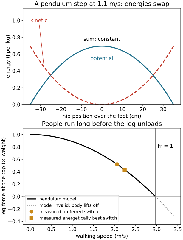
one pendulum step: the hip rises 7.1 cm, speed 1.10 m/s at the top, 1.61 m/s at the ends
kinetic and potential energy trade places; their sum changes by 0.0 J/kg
fastest possible walk (Fr = 1): v = √(g·L) = 2.97 m/s = 10.7 km/h
predicted switch to running at Fr = 0.5: 2.10 m/s
measured preferred switch: 2.06 m/s → Fr = 0.48, leg force at the top = 0.52 × body weight
measured energetically best switch: 2.24 m/s → Fr = 0.57, leg force at the top = 0.43 × body weight
What the result teaches:
- The pendulum trades energy for free. In the model, the hip rises by 7.1 cm, slows down to 1.10 m/s at the top and speeds up to 1.61 m/s at the ends of the step, while the sum of the energies does not change. Real walkers recover only part of the energy – up to 70 % 1 – because every step-to-step transition costs work 4.
- A speed limit. The fastest possible walk of the pendulum is 2.97 m/s, or 10.7 km/h. This is an upper limit of the model, not a measured top speed.
- People switch early. At Fr = 0.5, the model predicts the switch at 2.10 m/s; the measured preferred switch speed of 2.06 m/s corresponds to Fr = 0.48 – for the assumed leg length. At that speed, the leg still carries 0.52 times the body weight at the top of the arc: people start running long before the pendulum would lift off.
Try it yourself:
- A child with a leg length of 0.5 m: set
LEG = 0.50. The fastest walk drops to 2.21 m/s and the predicted switch to 1.57 m/s – a child has to start running sooner. - Walk on the Moon: set
G = 1.62. The fastest walk drops to 1.21 m/s, and if the switch still happens at Fr = 0.5, it would come at 0.85 m/s. This is an extrapolation: Kram and colleagues simulated reduced gravity on Earth, by pulling their subjects upwards, not on the Moon 11.
Where the output shows a negative leg force for a measured adult switch speed, that speed lies beyond Fr = 1 for the changed leg or gravity: the pendulum model no longer applies there.
Tested output with LEG = 0.50
one pendulum step: the hip rises 14.3 cm, speed 1.10 m/s at the top, 2.00 m/s at the ends
kinetic and potential energy trade places; their sum changes by 0.0 J/kg
fastest possible walk (Fr = 1): v = √(g·L) = 2.21 m/s = 8.0 km/h
predicted switch to running at Fr = 0.5: 1.57 m/s
measured preferred switch: 2.06 m/s → Fr = 0.87, leg force at the top = 0.13 × body weight
measured energetically best switch: 2.24 m/s → Fr = 1.02, leg force at the top = -0.02 × body weight
Tested output with G = 1.62
one pendulum step: the hip rises 7.1 cm, speed 1.10 m/s at the top, 1.20 m/s at the ends
kinetic and potential energy trade places; their sum changes by 0.0 J/kg
fastest possible walk (Fr = 1): v = √(g·L) = 1.21 m/s = 4.3 km/h
predicted switch to running at Fr = 0.5: 0.85 m/s
measured preferred switch: 2.06 m/s → Fr = 2.91, leg force at the top = -1.91 × body weight
measured energetically best switch: 2.24 m/s → Fr = 3.44, leg force at the top = -2.44 × body weight
Physical AI lens: robots that walk
Physical AI – robots that sense and act in the physical world – has to solve the problem every toddler solves: how to stay upright on two legs and move forward without falling. Engineers have tried two very different routes: build the physics into the machine, or let the machine learn.
Walking without a motor. In 1990, Tad McGeer described a class of two-legged machines for which walking is a natural motion. Started on a shallow slope, such a machine settles into a steady gait quite comparable to human walking – without motors, control or energy input other than gravity 14. These passive dynamic walkers are inverted pendulums built from rigid parts connected by joints. In 2005, Steven Collins, Andy Ruina, Russ Tedrake and Martijn Wisse presented three robots based on this idea, in which small active power sources took the place of the slope. They walked on level ground with less control and less energy than other powered robots, and more naturally – which suggests that passive dynamics are important in human walking, too 15.
A robot on a spring. The spring of the running leg also found its way into machines. In 1984, Marc Raibert and colleagues built a robot that hopped and ran on one springy leg and kept its balance on an open floor without support. Its control was split into three simple parts: one for the forward speed, one for the posture of the body and one for the hopping height 16.
Learning by trial and error. Today, many legged robots learn to move with reinforcement learning: a neural network controls a simulated robot, receives a reward for good behaviour and improves by trial and error over many simulated attempts. Jemin Hwangbo and colleagues trained such a network in simulation and transferred it to the four-legged robot ANYmal, the size of a medium dog. The learned controller followed speed commands more precisely and more energy-efficiently than the previous one, ran faster than before and got up after falls. According to the authors’ preprint, it beat the robot’s previous speed record by 25 %, and each training session took at most eleven hours on a personal computer 17.
Humanoid robots. Ilija Radosavovic and colleagues trained a controller for a full-size humanoid robot entirely in simulation – in many randomised virtual environments – and transferred it to the real robot without further training. The controller is a transformer, a type of neural network also used in large language models; it reads the recent history of the robot’s own sensor readings and actions and predicts the next action. The robot walked over various outdoor terrains and was robust to external disturbances 18. According to the authors’ preprint, the robot is about 1.6 m tall and weighs 45 kg, the simulation ran thousands of environments at once, the disturbances included pushes with a stick, and in a week of full-day tests outdoors no falls were observed 18. On a much smaller scale, Tuomas Haarnoja and colleagues trained miniature humanoids – 51 cm tall according to the preprint – to play one-against-one football. With the learned skills, the robots walked 181 % faster, turned 302 % faster and took 63 % less time to get up than with the robot’s scripted motions 19.
From pendulum to policy. The two routes meet: a learning robot moves in a simulated world that obeys the same physics of pendulums and springs, and a robot that uses this physics – like the passive walkers – needs less energy and less control. A review by Yuchuan Tong and colleagues lists what humanoid robots still lack: a deeper understanding of biological movement, better mechanical structures and materials, better drives and control, and more efficient use of energy 20.
What comes next
Humanoid robots that operate on their own in everyday surroundings “have the potential to help address labor shortages in factories, assist elderly at home, and colonize new planets” – this is how Radosavovic and colleagues describe their goal 18. It is a scenario, not a forecast: the review by Tong and colleagues names energy efficiency, drives, materials and control among the open challenges, and sees a promising direction in combining bionics, brain-inspired intelligence, mechanics and control 20.
Nature still sets the standard. Human walking combines a pendulum that trades energy almost for free, springs that return energy at every step and a nervous system that keeps the whole thing upright on uneven ground. Open questions remain on both sides: what exactly makes people switch from walking to running below the pendulum’s limit 13, and how robots can learn to walk with the economy of a human – or of a passive machine that walks down a slope with no motor at all 15.
Frequently asked questions
Why is walking compared to an inverted pendulum?
During each step, the stance leg stays almost straight, and the body vaults over it like a weight on top of a stiff rod. The body is lowest and fastest at the start and end of the step and highest and slowest in the middle. Kinetic energy is turned into potential energy and back, as in a pendulum, so the muscles have to supply only part of the energy.
Why do we start running when we walk faster?
In the pendulum model, gravity must pull the body round its arc over the foot. The faster you walk, the more pull you need, and at a Froude number of 1 gravity is no longer enough. People switch to running well before that, at a Froude number of about 0.5 – for adults around 2 metres per second. Why exactly at that point is still debated; it is not simply where running becomes cheaper.
What is the Froude number?
The Froude number Fr = v²/(gL) compares the centripetal acceleration of a body moving at speed v on a curve of radius L with the acceleration of gravity g. For walking, L is the leg length. Animals of different size move in a similar way when their Froude numbers are equal – a child and an adult, a dog and a horse.
How does the Achilles tendon save energy?
The Achilles tendon connects the calf muscles to the heel. When the foot is loaded, the tendon stretches like a rubber band and stores elastic energy, which it returns when the foot pushes off. In walking, the tendon stretches by several millimetres while the calf muscle hardly changes its length; in one-legged hopping, its recoil supplies on average about 16 % of the work of each hop.
How do humanoid robots learn to walk?
Many modern legged robots learn to walk with reinforcement learning: a neural network controls a simulated robot, gets a reward for walking well and improves by trial and error over many simulated runs. The trained network is then transferred to the real robot. Earlier approaches used carefully designed models and controllers; very efficient walkers even use the passive pendulum dynamics of their legs.
Sources
- Cavagna, G. A., Heglund, N. C., Taylor, C. R. (1977). Mechanical work in terrestrial locomotion: two basic mechanisms for minimizing energy expenditure. American Journal of Physiology – Regulatory, Integrative and Comparative Physiology 233, R243–R261. doi:10.1152/ajpregu.1977.233.5.r243
- Saibene, F., Minetti, A. E. (2003). Biomechanical and physiological aspects of legged locomotion in humans. European Journal of Applied Physiology 88, 297–316. doi:10.1007/s00421-002-0654-9
- Bramble, D. M., Lieberman, D. E. (2004). Endurance running and the evolution of Homo. Nature 432, 345–352. doi:10.1038/nature03052
- Kuo, A. D., Donelan, J. M., Ruina, A. (2005). Energetic Consequences of Walking Like an Inverted Pendulum: Step-to-Step Transitions. Exercise and Sport Sciences Reviews 33, 88–97. doi:10.1097/00003677-200504000-00006
- Kuo, A. D. (2007). The six determinants of gait and the inverted pendulum analogy: A dynamic walking perspective. Human Movement Science 26, 617–656. doi:10.1016/j.humov.2007.04.003
- Fukunaga, T., Kubo, K., Kawakami, Y., Fukashiro, S., Kanehisa, H., Maganaris, C. N. (2001). In vivo behaviour of human muscle tendon during walking. Proceedings of the Royal Society of London. Series B: Biological Sciences 268, 229–233. doi:10.1098/rspb.2000.1361 · Open Access
- Ker, R. F., Bennett, M. B., Bibby, S. R., Kester, R. C., Alexander, R. M. (1987). The spring in the arch of the human foot. Nature 325, 147–149. doi:10.1038/325147a0
- Lichtwark, G. A., Wilson, A. M. (2005). In vivo mechanical properties of the human Achilles tendon during one-legged hopping. Journal of Experimental Biology 208, 4715–4725. doi:10.1242/jeb.01950 · Open Access
- Alexander, R. M. (1984). The Gaits of Bipedal and Quadrupedal Animals. The International Journal of Robotics Research 3, 49–59. doi:10.1177/027836498400300205
- Blickhan, R. (1989). The spring-mass model for running and hopping. Journal of Biomechanics 22, 1217–1227. doi:10.1016/0021-9290(89)90224-8
- Kram, R., Domingo, A., Ferris, D. P. (1997). Effect of Reduced Gravity on the Preferred Walk–Run Transition Speed. Journal of Experimental Biology 200, 821–826. doi:10.1242/jeb.200.4.821
- Alexander, R. M., Jayes, A. S. (1983). A dynamic similarity hypothesis for the gaits of quadrupedal mammals. Journal of Zoology 201, 135–152. doi:10.1111/j.1469-7998.1983.tb04266.x
- Hreljac, A. (1993). Preferred and energetically optimal gait transition speeds in human locomotion. Medicine & Science in Sports & Exercise 25, 1158–1162. doi:10.1249/00005768-199310000-00012
- McGeer, T. (1990). Passive Dynamic Walking. The International Journal of Robotics Research 9, 62–82. doi:10.1177/027836499000900206
- Collins, S., Ruina, A., Tedrake, R., Wisse, M. (2005). Efficient Bipedal Robots Based on Passive-Dynamic Walkers. Science 307, 1082–1085. doi:10.1126/science.1107799
- Raibert, M. H., Brown, H. B., Chepponis, M. (1984). Experiments in Balance with a 3D One-Legged Hopping Machine. The International Journal of Robotics Research 3, 75–92. doi:10.1177/027836498400300207
- Hwangbo, J., Lee, J., Dosovitskiy, A., Bellicoso, D., Tsounis, V., Koltun, V., Hutter, M. (2019). Learning agile and dynamic motor skills for legged robots. Science Robotics 4, eaau5872. doi:10.1126/scirobotics.aau5872 · Open Access
- Radosavovic, I., Xiao, T., Zhang, B., Darrell, T., Malik, J., Sreenath, K. (2024). Real-world humanoid locomotion with reinforcement learning. Science Robotics 9, eadi9579. doi:10.1126/scirobotics.adi9579
- Haarnoja, T., Moran, B., Lever, G., Huang, S. H., Tirumala, D., Humplik, J., Wulfmeier, M., Tunyasuvunakool, S., Siegel, N. Y., Hafner, R., Bloesch, M., Hartikainen, K., Byravan, A., Hasenclever, L., Tassa, Y., Sadeghi, F., Batchelor, N., Casarini, F., Saliceti, S., Game, C., Sreendra, N., Patel, K., Gwira, M., Huber, A., Hurley, N., Nori, F., Hadsell, R., Heess, N. (2024). Learning agile soccer skills for a bipedal robot with deep reinforcement learning. Science Robotics 9, eadi8022. doi:10.1126/scirobotics.adi8022 · Open Access
- Tong, Y., Liu, H., Zhang, Z. (2024). Advancements in Humanoid Robots: A Comprehensive Review and Future Prospects. IEEE/CAA Journal of Automatica Sinica 11, 301–328. doi:10.1109/jas.2023.124140
Text and figures: CC BY-SA 4.0. Found a mistake? Open an issue or edit this article on GitHub.