Life where water feels like honey
Imagine you are as small as a bacterium. Water, which carries a swimmer and lets a boat glide, suddenly behaves like a thick syrup. If you stop paddling, you do not glide on – you stop at once. The physicist Edward Purcell described this world in a famous lecture in 1976, reprinted in 1977: for a bacterium, inertia plays no role whatsoever; what it does at any moment is set only by the forces acting on it at that moment 1.
Purcell’s picture was vivid. To swim the way a microorganism does, you would have to be in a swimming pool full of molasses – and you would not be allowed to move any part of your body faster than 1 cm per minute. If under these rules you managed to move a few metres in a couple of weeks, you would qualify as a low-Reynolds-number swimmer 1. Honey would serve almost as well as molasses: even a runny rosemary honey, measured at 30 °C, is about 6,000 times as viscous as water with its 1 mPa·s 2 1. But, as the physics lens shows, a thick liquid alone is not enough – the slowness matters just as much.
This is the world of the overwhelming majority of organisms 1. Microorganisms such as the gut bacterium Escherichia coli swim in it every second 1 3. This article explains how they do it – and why tiny robots are now being built after their example.
A run and a tumble in three steps
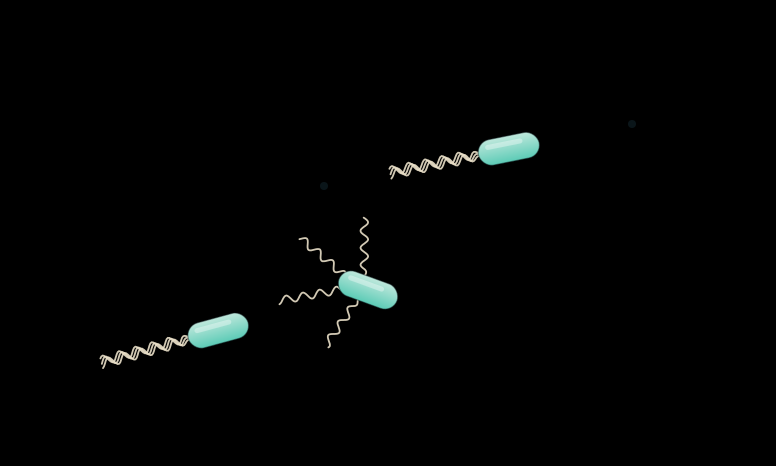
- Run. Several thin, helical flagella rotate at about 100 revolutions per second 4 5. They bundle together and push the cell forward like a corkscrew, at typically 20–40 µm per second, for a second or two 1.
- Tumble. One or more motors reverse, the flagella no longer turn together, and the cell tumbles in place. A single reversing flagellum can be enough to trigger a tumble 5.
- New direction. The cell sets off on a new run in a new direction. If things are getting better – more food – it runs longer before it tumbles again 1.
Biology lens: a rotary motor and a sense of smell
E. coli is a rod-shaped bacterium about 2 µm long 1. It carries several flagella; each is several micrometres long but only about 20 nanometres thick 5. For a long time it was thought that such flagella wave like a tail. In 1973, Howard Berg and Robert Anderson argued that bacteria swim by rotating their flagellar filaments 4, and experiments soon confirmed it: when the hook at the base of a flagellum was glued to a microscope slide, the whole cell body rotated at constant speed 1. At the base of each flagellum sits a true rotary motor, and it can turn in both directions 1.
The direction of the motors decides between running and tumbling. When the filaments are filmed in real time, tumbles turn out to be remarkably varied: not every flagellum has to reverse, and a tumble can result from the reversal of just one 5. During a tumble the filaments change their shape as well – they switch between different helical forms 5.
Why swim at all? Not to stir the water: for a bacterium, food arrives by diffusion, and stirring around the cell accomplishes nothing 1. Swimming pays off in a different way – it carries the cell to places where food is more abundant. Berg tracked single bacteria in three dimensions and found that they gradually work their way up a gradient of attractant. The rule they follow is simple: if things are getting better, don’t stop so soon 1. Runs up the gradient get longer; runs down the gradient do not get shorter 1.
To follow a gradient, a cell must measure concentrations. Berg and Purcell calculated the precision that is physically possible for a cell that counts molecules with receptors on its surface – and found that the chemotactic sensitivity of E. coli approaches that of a cell of optimum design 6. This ability to move according to chemical signals is called chemotaxis.
Physics lens: when viscosity beats inertia
Whether a swimmer glides or stops at once is decided by a single dimensionless number, the Reynolds number. It compares the inertial forces in a flow with the viscous forces 1:
Here ρ is the density of the liquid, η its viscosity, v the speed of the swimmer and L its size. For E. coli – of the order of 1 µm in size, swimming at 30 µm/s in water – Purcell estimated Re ≈ 3 × 10⁻⁵ 1. At such values the inertia terms of the Navier–Stokes equation can be dropped; what remains describes Stokes flow, and it has no memory 1 3.
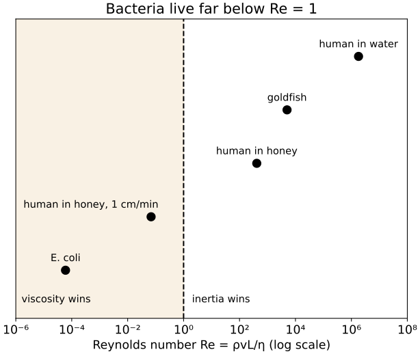
The program below calculates the Reynolds number for a few swimmers and asks the honey question: how close does a human in honey come to the world of a bacterium? Size, speed and the density of honey are rough typical values chosen for illustration; the viscosity of honey is the measured value for a runny rosemary honey at 30 °C 2, the viscosity of water 1 mPa·s 1.
import numpy as np
import matplotlib.pyplot as plt

# Fluids: density (kg/m³) and viscosity (Pa·s)
WATER = (1000, 1.0e-3)       # water: viscosity 1 mPa·s
HONEY = (1400, 6.1)          # runny honey: 6.1 Pa·s (rosemary honey, 30 °C); density assumed
COLI_FLUID = WATER           # the liquid E. coli swims in
# Swimmers: (name, size L in m, speed v in m/s, fluid) – rough typical values, see the text
SWIMMERS = [
    ("human in water", 1.8, 1.0, WATER),
    ("goldfish", 0.05, 0.1, WATER),
    ("human in honey", 1.8, 1.0, HONEY),
    ("human in honey, 1 cm/min", 1.8, 0.01 / 60, HONEY),
    ("E. coli", 2e-6, 30e-6, COLI_FLUID),
]


def reynolds(size, speed, fluid):
    """Re = ρ·v·L/η: inertial forces divided by viscous forces."""
    density, viscosity = fluid
    return density * speed * size / viscosity


for name, size, speed, fluid in SWIMMERS:
    print(f"{name:26s} Re = {reynolds(size, speed, fluid):8.1g}")

# How far does E. coli coast when its motor stops? A sphere of radius a in a viscous fluid
# slows down exponentially with the time constant τ = m / (6πηa) (Stokes drag).
radius, speed, cell_density = 1e-6, 30e-6, 1000      # m, m/s, kg/m³ (cell ≈ water)
mass = cell_density * 4 / 3 * np.pi * radius**3
tau = mass / (6 * np.pi * WATER[1] * radius)
print(f"E. coli stops within {tau * 1e6:.1g} µs and coasts {speed * tau * 1e10:.1g} Å "
      f"(an atom is roughly 1 Å across)")

SUPERSCRIPT = str.maketrans("-0123456789", "⁻⁰¹²³⁴⁵⁶⁷⁸⁹")


def power_of_ten(value, _pos=None):
    """Tick label 10⁻⁴ as plain text (no mathtext)."""
    return "10" + str(int(round(np.log10(value)))).translate(SUPERSCRIPT)


names = [s[0] for s in SWIMMERS]
values = [reynolds(*s[1:]) for s in SWIMMERS]
plt.rcParams["font.size"] = 13      # large type: the chart stays readable on a phone
fig, ax = plt.subplots(figsize=(6.4, 5.4), layout="constrained")
ax.axvspan(1e-6, 1, color="#c98a1b", alpha=0.12)
ax.axvline(1, color="black", lw=1.5, ls="--")
ax.text(1.6e-6, 4.6, "viscosity wins", fontsize=11)
ax.text(2, 4.6, "inertia wins", fontsize=11)
for row, (name, value) in enumerate(zip(names, values)):
    ax.plot(value, row, "o", ms=9, color="black")
    near_line = 1e-3 < value < 1        # keep this label left of the dashed line
    ax.annotate(name, (value, row), xytext=(8 if near_line else 0, 10), textcoords="offset points",
                ha="right" if near_line else "center", fontsize=11)
ax.set_xscale("log")
ax.set_xlim(1e-6, 1e8)
ax.set_ylim(4.9, -0.7)
ax.set_yticks([])
ax.xaxis.set_major_locator(plt.LogLocator(numticks=8))
ax.xaxis.set_major_formatter(power_of_ten)
ax.set_xlabel("Reynolds number Re = ρvL/η (log scale)")
ax.set_title("Bacteria live far below Re = 1")
plt.show()
Output · what the code prints, re-run at every build
human in water             Re =    2e+06
goldfish                   Re =    5e+03
human in honey             Re =    4e+02
human in honey, 1 cm/min   Re =     0.07
E. coli                    Re =    6e-05
E. coli stops within 0.2 µs and coasts 0.07 Å (an atom is roughly 1 Å across)
What the result teaches:
- Honey alone is not enough. A human swimming normally in honey still reaches Re ≈ 400 – inertia still matters. Only when the swimmer also slows down to 1 cm per minute, as in Purcell’s rule, does the Reynolds number fall below 1 (0.07).
- The bacterium is in a world of its own. At Re ≈ 6 × 10⁻⁵ – twice Purcell’s value, because the program uses the cell’s length of 2 µm – E. coli lies more than a thousand times below even the slow human in honey. Our estimate for a swimming human, 2 × 10⁶, is higher than Purcell’s rough value of 104 1; what counts is the order of magnitude, and with a body length of 1.8 m and 1 m/s the formula gives millions.
- No coasting. When its motor stops, the bacterium comes to rest within 0.2 µs and coasts 0.07 Å – a fraction of the width of an atom. Purcell gave the same order of magnitude: about 0.1 Å in well under a microsecond 1.
Try it yourself:
- Put E. coli into honey: set
COLI_FLUID = HONEY. Its Reynolds number drops to 1e-08 – but for the bacterium almost nothing changes: it was deep in the viscous world already. - Let the human swim at 1 cm per second instead of per minute: change
0.01 / 60to0.01. The Reynolds number rises to 4 – above 1 again.
Tested output with COLI_FLUID = HONEY
human in water             Re =    2e+06
goldfish                   Re =    5e+03
human in honey             Re =    4e+02
human in honey, 1 cm/min   Re =     0.07
E. coli                    Re =    1e-08
E. coli stops within 0.2 µs and coasts 0.07 Å (an atom is roughly 1 Å across)
Tested output with 0.01
human in water             Re =    2e+06
goldfish                   Re =    5e+03
human in honey             Re =    4e+02
human in honey, 1 cm/min   Re =        4
E. coli                    Re =    6e-05
E. coli stops within 0.2 µs and coasts 0.07 Å (an atom is roughly 1 Å across)
The scallop theorem. Because time drops out of Stokes flow, a swimmer that simply reverses its stroke goes nowhere. Purcell’s example is a scallop: it opens its shell slowly and closes it fast, but with only one hinge it can only move back and forth – and at low Reynolds number it would end exactly where it started, however fast or slowly it moves 1. A microswimmer needs a motion that is not reversible: a flexible oar that bends one way on the stroke and the other way on the way back, or a corkscrew that keeps turning 1.
How a corkscrew pushes. A viscous liquid resists a thin filament more strongly when it moves sideways than when it moves along its length 1 3. This difference turns rotation into thrust: a helix that is made to rotate necessarily translates, and a helix that is pulled along necessarily rotates 7. Purcell estimated that a sphere driven by such a helical propeller converts only about 1 % of the motor’s work into useful propulsion 1. For the bacterium it hardly matters: swimming at 30 µm/s costs it about 0.5 W per kilogram, a small fraction of its energy budget 1.
Mathematics lens: a random walk with a bias
Outrunning diffusion. Food molecules spread by diffusion. In a time t they get about √(D t) far, where D is their diffusion constant – for typical small molecules in water about 10−5 cm2/s, or 1,000 µm2/s 1. Swimming carries the cell a distance ℓ in a time ℓ/v; diffusion needs about ℓ2/D. Swimming wins only when
With v = 30 µm/s this gives about 30 µm – roughly the length of a bacterial run. As Purcell put it: a bacterium that does not swim that far has not gone anywhere 1.
A run-and-tumble walk spreads like diffusion. Model the bacterium in two dimensions: it runs at speed v, each run lasts a random time with mean τ, and each tumble chooses a completely new direction. Run durations of this kind follow an exponential distribution, for which the mean square of the duration is 2τ2. One run therefore covers a mean square distance of 2v2τ2, and in a time t there are about t/τ independent runs:
With v = 20 µm/s and τ = 1 s, D = 200 µm2/s – a population of swimming bacteria spreads about five times more slowly than a small molecule diffuses.
The bias. Now let runs that point up the gradient (towards +x) last b times longer on average. After a tumble, the new direction points up the gradient with probability ½. Weighted by their duration, runs up the gradient take a fraction b/(1 + b) of the time, runs down the gradient 1/(1 + b). Averaged over all directions of one half, the component of the velocity along x is (2/π) v. The drift speed is therefore
For b = 2 – runs up the gradient last twice as long – the drift is (2/π) · (1/3) ≈ 21 % of the swimming speed. The computer science lens checks this result with a simulation.
Computer science lens: run and tumble as an algorithm
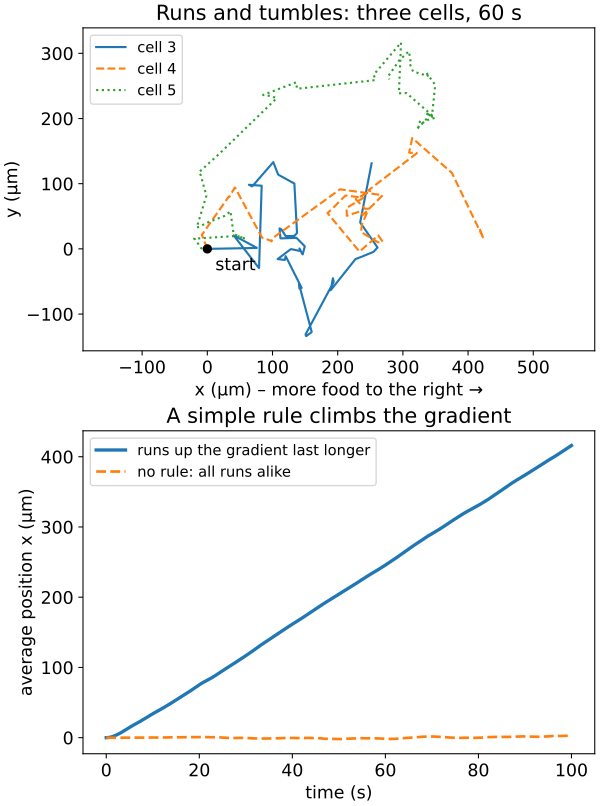
The bacterium has no map and no brain. It cannot even sense in which direction the food lies – it only notices whether things are getting better over time. Its search algorithm fits in one line: if things are getting better, don’t stop so soon 1. The program below simulates 2,000 bacteria with and without this rule. The speed of 20 µm/s lies in the range Berg measured 1; the mean run time of 1 s, the factor 2 for runs up the gradient and the completely random new direction after each tumble are model assumptions.
import numpy as np
import matplotlib.pyplot as plt

# Model parameters – typical values, see the article
SPEED = 20.0       # swimming speed during a run (µm/s); Berg measured 20–40 µm/s
RUN_TIME = 1.0     # mean run duration (s) when nothing improves
BOOST = 2.0        # runs up the food gradient last BOOST times longer on average
N_CELLS = 2000     # bacteria per population
T_END = 100.0      # simulated time (s)
DT = 0.01          # time step (s)
rng = np.random.default_rng(1)


def swim(boost):
    """Run and tumble in 2D. Food increases towards +x, so 'getting better' means moving to +x.

    A tumble is instantaneous and picks a completely random new direction (a simplification).
    In each step a cell tumbles with probability DT / mean run time. Berg's rule: if things are
    getting better, don't stop so soon – runs towards +x use RUN_TIME × boost.
    """
    steps = int(T_END / DT)
    angle = rng.uniform(0, 2 * np.pi, N_CELLS)
    track = np.zeros((steps + 1, N_CELLS, 2))
    for i in range(steps):
        heading = np.column_stack((np.cos(angle), np.sin(angle)))
        track[i + 1] = track[i] + SPEED * DT * heading
        mean_run = np.where(heading[:, 0] > 0, RUN_TIME * boost, RUN_TIME)
        tumble = rng.random(N_CELLS) < DT / mean_run
        angle = np.where(tumble, rng.uniform(0, 2 * np.pi, N_CELLS), angle)
    return track


t = np.arange(int(T_END / DT) + 1) * DT
late = t > 20                     # fit after the first runs, when the walk has lost its start
plain = swim(boost=1.0)
biased = swim(boost=BOOST)

# 1) No gradient: a random walk. Its spreading follows <r²> = 4 D t with D = v² τ / 2 in 2D.
msd = (plain ** 2).sum(axis=2).mean(axis=1)
d_sim = np.polyfit(t[late], msd[late], 1)[0] / 4
print(f"random walk: D = {d_sim:.0f} µm²/s (formula v²τ/2 = {SPEED**2 * RUN_TIME / 2:.0f} µm²/s)")

# 2) Berg's rule: the population drifts up the gradient. Formula: v · (2/π) · (b − 1)/(b + 1).
drift_sim = np.polyfit(t[late], biased[late, :, 0].mean(axis=1), 1)[0]
drift_theory = SPEED * 2 / np.pi * (BOOST - 1) / (BOOST + 1)
# round(...) + 0.0 turns a rounded "-0.0" into "0.0"
print(f"with the rule: drift {round(drift_sim, 1) + 0.0} µm/s (formula {drift_theory:.1f} µm/s), "
      f"{round(100 * drift_sim / SPEED) + 0} % of the swimming speed")
print(f"after {T_END:.0f} s the average cell is {biased[-1, :, 0].mean():.0f} µm further up the gradient")

plt.rcParams["font.size"] = 13      # large type: the chart stays readable on a phone
fig, (top, bottom) = plt.subplots(2, 1, figsize=(6.4, 8.4), layout="constrained")
for k, style in zip(range(3, 6), ["-", "--", ":"]):   # three of the cells, first 60 s
    path = biased[: int(60 / DT) : 5, k]
    top.plot(path[:, 0], path[:, 1], style, lw=1.6, label=f"cell {k}")
top.plot(0, 0, "ko", ms=6)
top.annotate("start", (0, 0), textcoords="offset points", xytext=(6, -16))
top.set_aspect("equal", adjustable="datalim")
top.set_xlabel("x (µm) – more food to the right →")
top.set_ylabel("y (µm)")
top.set_title("Runs and tumbles: three cells, 60 s")
top.legend(loc="upper left", fontsize=11)

bottom.plot(t, biased[..., 0].mean(axis=1), lw=2.5, label="runs up the gradient last longer")
bottom.plot(t, plain[..., 0].mean(axis=1), "--", lw=2, label="no rule: all runs alike")
bottom.set_xlabel("time (s)")
bottom.set_ylabel("average position x (µm)")
bottom.set_title("A simple rule climbs the gradient")
bottom.legend(loc="upper left", fontsize=11)
plt.show()
Output · what the code prints, re-run at every build
random walk: D = 195 µm²/s (formula v²τ/2 = 200 µm²/s)
with the rule: drift 4.3 µm/s (formula 4.2 µm/s), 21 % of the swimming speed
after 100 s the average cell is 416 µm further up the gradient
What the result teaches:
- The simulation agrees with the mathematics. Without the rule, the bacteria spread with D ≈ 195 µm2/s; the formula v2τ/2 gives 200 µm2/s. With the rule, the population drifts at 4.3 µm/s; the formula of the mathematics lens gives 4.2 µm/s. The small differences are random and change with the seed.
- A weak bias is enough. No single cell swims straight to the food; each path looks like a random zigzag. Yet the population drifts at about a fifth of the swimming speed and after 100 s is on average 416 µm further up the gradient.
- Only time is compared, not space. The program never uses the direction of the gradient to steer – only to decide whether things are getting better. That is all a cell of 2 µm can measure.
Try it yourself:
- Set
BOOST = 1.0: the rule is switched off, the drift falls to 0.0 µm/s. - Set
BOOST = 4.0: runs up the gradient last four times as long, and the drift rises to about 7.6 µm/s – the formula predicts 7.6 µm/s.
Tested output with BOOST = 1.0
random walk: D = 195 µm²/s (formula v²τ/2 = 200 µm²/s)
with the rule: drift 0.0 µm/s (formula 0.0 µm/s), 0 % of the swimming speed
after 100 s the average cell is -5 µm further up the gradient
Tested output with BOOST = 4.0
random walk: D = 195 µm²/s (formula v²τ/2 = 200 µm²/s)
with the rule: drift 7.6 µm/s (formula 7.6 µm/s), 38 % of the swimming speed
after 100 s the average cell is 746 µm further up the gradient
From bacteria to robots. The same algorithm works for machines that look for the source of a signal. Amit Dhariwal and colleagues developed robots that navigate to the source of a signal with a biased random walk inspired by chemotaxis, tested it in extensive simulations and on a small robot that followed light. In their comparison, gradient descent – always moving in the direction of the steepest increase – was faster, but the bacterial strategy performed better with multiple sources and with sources that dissipate, and it was better suited to covering the boundary of a region 8.
Physical AI lens: microrobots after the bacterial flagellum
For Physical AI – robots that sense and act in the real world – the bacterium is a special role model. A robot the size of a bacterium faces the bacterium’s physics: no inertia, no gliding, and the scallop theorem forbids every simple back-and-forth stroke 1 3. Engineers have therefore copied nature’s two solutions.
The corkscrew. In 2009, Li Zhang, Bradley Nelson and colleagues built artificial bacterial flagella: a helical tail with the shape and size of a natural flagellum and a thin soft-magnetic “head” at one end. Weak magnetic fields from three pairs of electromagnetic coils drive and steer the swimmer; the authors describe it as the first demonstration of microscopic artificial swimmers with helical propulsion. They could push microspheres around 9. In the same year, Ambarish Ghosh and Peer Fischer showed chiral propellers made of nanostructured surfaces that can be produced in large numbers and steered through water with micrometre precision by homogeneous magnetic fields; they can carry chemicals and push loads 10.
The flexible oar. Rémi Dreyfus and colleagues linked magnetic particles with DNA into a flexible chain and attached it to a red blood cell. An oscillating magnetic field made the chain beat like a tail and propelled the structure; the fields controlled speed and direction 11.
Where is the intelligence? In these robots it sits outside: sensing, planning and steering are done by the coils and the computer that controls them, while the swimmer itself only converts the field into motion 12. The bacterium shows the other end of the scale – a body in which sensing, a simple decision rule and the motor are all built in. In our view, bringing more of that embodied intelligence into machines this small is one of the big open questions; Sitti and colleagues review the challenges of designing robots this small for work inside the body 13. Medicine is the main motivation: untethered, wirelessly controlled microrobots could make diagnosis and therapy less invasive and reach places in the body that are hard to access 12 13. This is still largely a research goal, not routine practice.
What we can learn from a bacterium
The bacterium shows how differently physics feels at another scale. Where we rely on momentum, it relies on friction; where we would stir, it waits for diffusion; where we would look ahead, it compares the present with the recent past. Its swimming machine – a rotary motor that turns a corkscrew – is inefficient by engineering standards and still perfectly good enough 1.
Many questions remain open: how flagella interact with each other and with nearby walls, how microorganisms swim in complex fluids such as mucus, and how to design artificial swimmers that work well at this scale are active fields of research 3. And for microrobots in medicine, the way from the laboratory into the body is still long 13.
Frequently asked questions
Why is water like honey for a bacterium?
What matters is not the liquid alone but the ratio of inertia to viscous friction, the Reynolds number. It depends on the size and speed of the swimmer. A bacterium is a few micrometres long and swims a few tens of micrometres per second, so its Reynolds number is only about 0.00003 to 0.00006, depending on whether its width or its length is taken as its size. Even in honey and moving no faster than 1 cm per minute, a human would still be about a thousand times above it; it would take an even thicker liquid and far slower movements.
How does E. coli swim?
E. coli has several thin, helical flagella. At the base of each sits a rotary motor that turns it about a hundred times per second. During a run the flagella bundle together and work like a corkscrew that pushes the cell forward. When a motor reverses, the flagella no longer turn together, the cell tumbles and then swims off in a new direction.
What is the scallop theorem?
At low Reynolds number, a swimmer that only opens and closes – like a scallop with a single hinge – goes nowhere: whatever it gains on one stroke it loses on the way back, however fast or slowly it moves. Microorganisms therefore use motions that are not reversible, such as a rotating corkscrew or a flexible, beating tail.
How do bacteria find food?
E. coli cannot steer directly. It swims in straight runs and changes direction at random in short tumbles. But it compares the concentration of food over time: if things are getting better, it runs longer before the next tumble. On average this biased random walk carries the bacterium towards more food.
What are bacteria-inspired microrobots?
They are artificial swimmers of the size of a bacterium, for example tiny magnetic corkscrews shaped like a bacterial flagellum. Weak magnetic fields from outside drive and steer them. They can push small particles or carry chemicals, and they are being developed for medicine, for example to deliver drugs; medical use is still a research goal.
Sources
- Purcell, E. M. (1977). Life at low Reynolds number. American Journal of Physics 45, 3–11. doi:10.1119/1.10903
- Afonso, M., Magalhães, M., Fernandes, L., Castro, M., Ramalhosa, E. (2018). Temperature effect on rheological behavior of Portuguese honeys. Polish Journal of Food and Nutrition Sciences 68, 217–222. doi:10.1515/pjfns-2017-0030 · Open Access
- Lauga, E., Powers, T. R. (2009). The hydrodynamics of swimming microorganisms. Reports on Progress in Physics 72, 096601. doi:10.1088/0034-4885/72/9/096601 · Open Access
- Berg, H. C., Anderson, R. A. (1973). Bacteria swim by rotating their flagellar filaments. Nature 245, 380–382. doi:10.1038/245380a0
- Turner, L., Ryu, W. S., Berg, H. C. (2000). Real-time imaging of fluorescent flagellar filaments. Journal of Bacteriology 182, 2793–2801. doi:10.1128/JB.182.10.2793-2801.2000 · Open Access
- Berg, H. C., Purcell, E. M. (1977). Physics of chemoreception. Biophysical Journal 20, 193–219. doi:10.1016/S0006-3495(77)85544-6 · Open Access
- Purcell, E. M. (1997). The efficiency of propulsion by a rotating flagellum. Proceedings of the National Academy of Sciences 94, 11307–11311. doi:10.1073/pnas.94.21.11307 · Open Access
- Dhariwal, A., Sukhatme, G. S., Requicha, A. A. G. (2004). Bacterium-inspired robots for environmental monitoring. Proceedings of the IEEE International Conference on Robotics and Automation (ICRA 2004) 2, 1436–1443. doi:10.1109/ROBOT.2004.1308026
- Zhang, L., Abbott, J. J., Dong, L., Kratochvil, B. E., Bell, D., Nelson, B. J. (2009). Artificial bacterial flagella: fabrication and magnetic control. Applied Physics Letters 94, 064107. doi:10.1063/1.3079655
- Ghosh, A., Fischer, P. (2009). Controlled propulsion of artificial magnetic nanostructured propellers. Nano Letters 9, 2243–2245. doi:10.1021/nl900186w
- Dreyfus, R., Baudry, J., Roper, M. L., Fermigier, M., Stone, H. A., Bibette, J. (2005). Microscopic artificial swimmers. Nature 437, 862–865. doi:10.1038/nature04090
- Nelson, B. J., Kaliakatsos, I. K., Abbott, J. J. (2010). Microrobots for minimally invasive medicine. Annual Review of Biomedical Engineering 12, 55–85. doi:10.1146/annurev-bioeng-010510-103409
- Sitti, M., Ceylan, H., Hu, W., Giltinan, J., Turan, M., Yim, S., Diller, E. (2015). Biomedical applications of untethered mobile milli/microrobots. Proceedings of the IEEE 103, 205–224. doi:10.1109/JPROC.2014.2385105
Text and figures: CC BY-SA 4.0. Found a mistake? Open an issue or edit this article on GitHub.